When working with sales data, it can be helpful to quickly identify which sales figures are doing well and which ones need improvement. Custom number formatting in Excel allows you to visually highlight data that meets certain criteria. In this article, we will show you how to use custom number formatting to highlight sales figures in red and green font with corresponding emojis.
What is Custom Number Formatting?
Custom number formatting allows you to change the way data is displayed in a cell without actually changing the underlying value. You can use custom number formatting to add symbols, change the color of text, and even add emojis to cells. Custom number formatting is based on a code that tells Excel how to display the data. The code consists of up to four parts, separated by semicolons. Each part corresponds to a different type of formatting, such as positive numbers, negative numbers, zero values, and text values.
Sales Data points
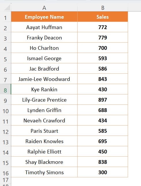
We have below given employee wise sales data in excel sheet-
Highlighting Sales with Red and Green font with Emojis
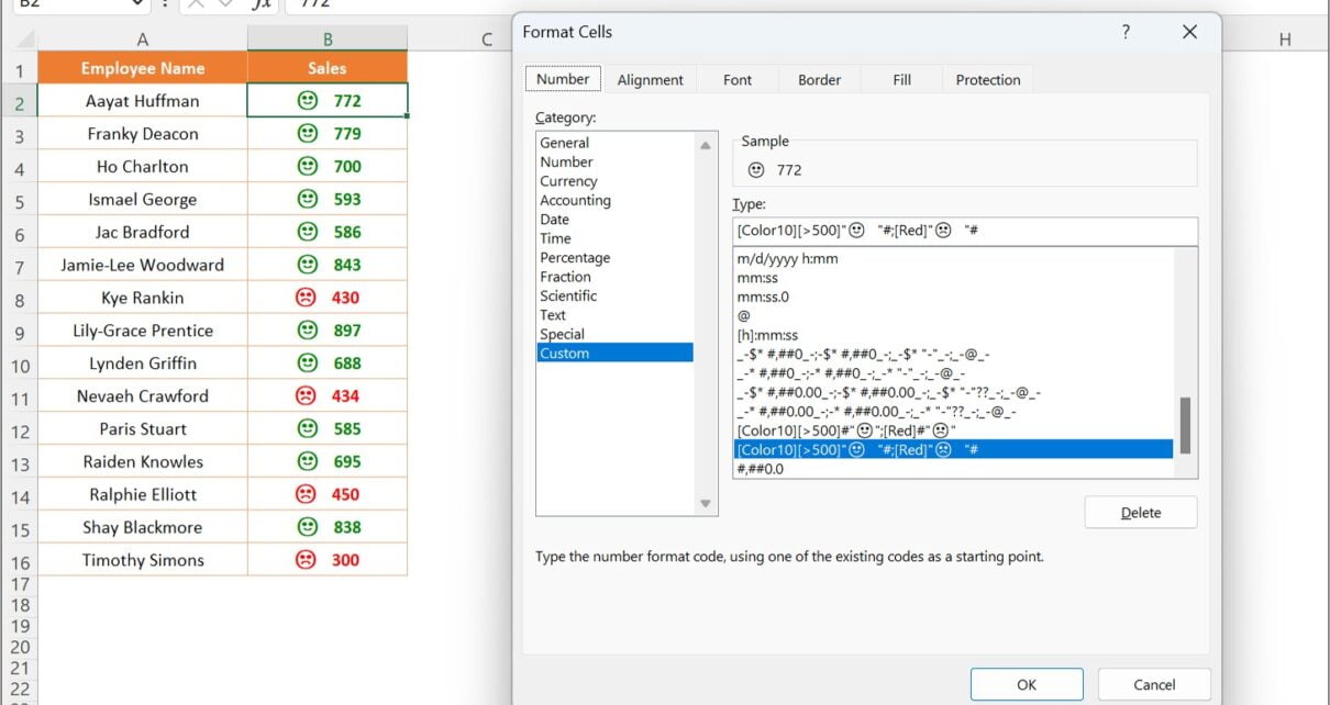
We will highlight sales figures which are less than or equal to 500 with red font and a sad emoji. Similarly, we will highlight sales figures which are greater than 500 with green font and a happy emoji.
we will use the following custom number format code:
[Color10][>500]"🙂 "#;[Red]"☹️ "#"
To apply this formatting to the Sales column, follow these steps:
- Select the Sales column.
- Right-click and select “Format Cells.”
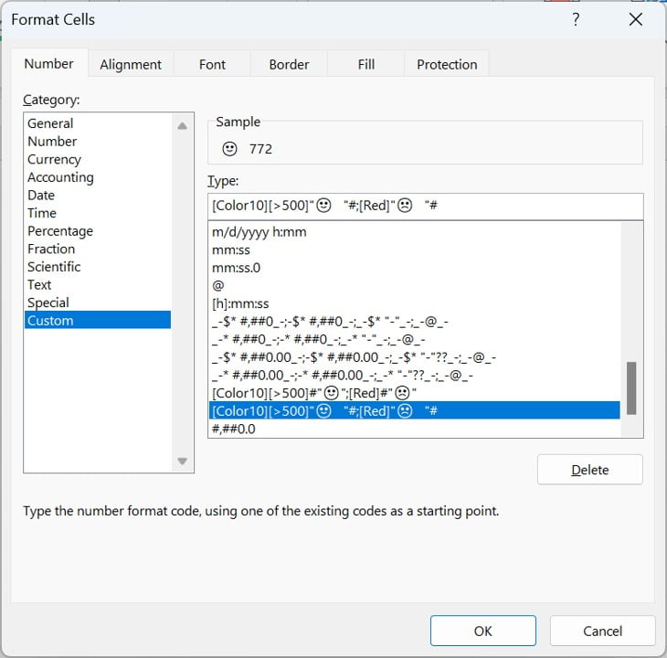
- In the Format Cells dialog box, select “Custom” from the Category list.
- In the Type field, enter the custom number format code shown above.
- Click “OK” to apply the formatting.
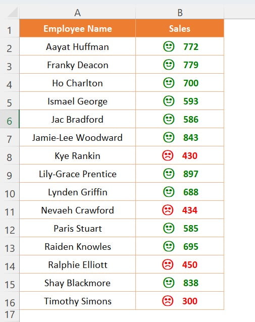
The Sales figures that are less than or equal to 500 will now be displayed in red font with a sad emoji. And, the Sales figures that are greater than 500 will now be displayed in green font with a happy emoji.
Tips for Using Custom Number Formatting Effectively
Here are some tips to keep in mind when using custom number formatting in Excel:
- Use colors and emojis sparingly to avoid overwhelming the data.
- Choose colors and emojis that are easy to understand and consistent with the message you want to convey.
- Test the custom number formatting on a small sample of data before applying it to the entire dataset.
- Make sure the custom number formatting does not interfere with any calculations or formulas you may have in the worksheet.
Conclusion
Custom number formatting in Excel is a powerful tool that can be used to highlight important data and make it more readable. By using custom number formatting to highlight sales figures with different colors and emojis, you can quickly identify which sales are doing well and which ones need improvement. Follow the steps outlined in this article to create custom number formats that highlight sales figures in red and green font with corresponding emojis.
Frequently Asked Questions
Q. Can I use different emojis with custom number formatting?
A. Yes, you can use any emoji which is available in your system. Use window+(.) shortcut key to open the windows emoji.
Q. How do I remove custom number formatting from a cell?
A. To remove custom number formatting from a cell, select the cell and right-click. Then select “Format Cells” and choose the “General” category in the Format Cells dialog box. Click “OK” to remove the custom number formatting.
Q. Can I apply custom number formatting to other types of data besides numbers?
A. Yes, you can apply custom number formatting to any type of data in Excel, including text and dates. Simply adjust the custom number format code to fit the data type you are working with.
Q. How can I modify an existing custom number format?
A. To modify an existing custom number format, select the cell with the custom number format and right-click. Then select “Format Cells” and choose the “Custom” category in the Format Cells dialog box. Edit the custom number format code in the Type field and click “OK” to apply the changes.
Q. Can I use conditional formatting with custom number formatting?
A. Yes, you can use conditional formatting to apply custom number formatting to specific cells or ranges of cells based on certain criteria. Follow the steps given in this article to apply custom number formatting.
Visit our YouTube channel to learn step-by-step video tutorials
Watch the step-by-step video tutorial:
Click here to download the practice file