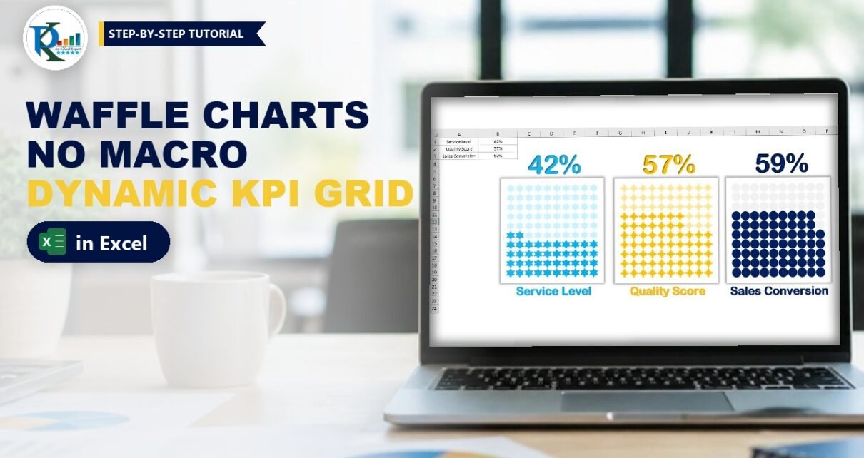
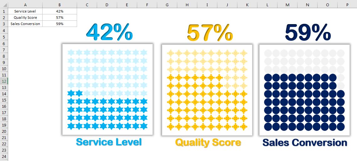
Waffle charts in Excel without macro are a smart way to show a percentage: a 10×10 grid where every cell is one percentage point, so 48% lights up 48 of the 100 shapes. They are perfect for KPI metrics like Service Level %, Quality Score %, Sales Conversion % or Project Completion %. In this tutorial you will build a fully dynamic waffle chart with two stacked column charts, a small helper sheet and a few shapes. There is no VBA at all: change the percentage and the chart updates by itself.
Watch the Video Tutorial
In the video, PK builds the Service Level waffle chart from a blank workbook: a helper grid of IF and SUM formulas, two 10-series stacked column charts, shapes pasted into the columns and a linked percentage label.
What You Will Build
- A Chart sheet with the KPI value and a Support sheet with a 10×10 formula grid.
- A background chart that always shows all 100 shapes in a light colour.
- A front chart that shows only the filled shapes in a dark colour, placed exactly on top of the background chart.
- A big percentage label linked to the cell, so the whole visual is dynamic.
How the Waffle Chart Works
The waffle is two stacked column charts with 10 columns and 10 series of 1s, which gives 100 equal blocks, each filled with a shape.
The background chart uses fixed values of 1, so all 100 shapes are always visible in a light colour. The front chart takes its values from a helper grid that returns 1 only for the filled cells, so the light shapes show through everywhere else.
The grid fills the bottom row first, from left to right, and then moves up, row by row.
Part 1: Set Up the Data for Waffle Charts in Excel
Step 1: Create the Chart and Support sheets
Open a new workbook with Ctrl + N. Name the first sheet Chart and add a second sheet named Support. On the Chart sheet type Service Level in A1 and your value in B1, for example 80%.
Step 2: Convert the percentage to a whole number
On the Support sheet type Service Level in A1 and this formula in B1:
=ROUND(Chart!B1*100,0)80% becomes 80, the number of shapes to fill. ROUND with 0 digits matters when your value has decimals: 80.35% would otherwise give 80.35, and the grid needs a whole number.
Step 3: Build the first column of the grid
Type 0 in Support!E1. In E2 enter:
=IF(SUM(E$1:E1)>=$B$1,"",1)Fill it down to E11, so the column has 10 formula cells.
Step 4: Add the running-total headers
In F1 enter:
=SUM($E$2:E11)Fill it right to N1. You now have 10 columns, E to N. Then copy E2:E11 and paste it into F2:N11. With 80 in B1, columns E to L are full of 1s and columns M and N are blank. The headers in row 1 read 0, 10, 20, 30 and so on.
How the formulas work
- Row 1 headers count how many 1s are already in all the columns to the left. E1 is 0 because nothing comes before column E. G1 is
=SUM($E$2:F11), the 1s in columns E and F. The$E$2start is locked and the end moves as you fill right. - The IF formula adds the header to the 1s above it in the same column:
SUM(E$1:E1)in E2,SUM(E$1:E2)in E3, and so on. That is the number of shapes already filled before this cell. - If that count has reached the target in
$B$1, the cell returns blank (""). Otherwise it returns 1. - So the grid contains exactly B1 ones. With 36, columns E, F and G are full (30) and column H has six 1s.
To test it, put =RANDBETWEEN(5,100)% in Chart!B1 and press F9: the 1s in the grid change every time.
Part 2: Create the Two Stacked Column Charts
Step 5: Insert a blank stacked column chart
Click an empty cell away from the data and go to Insert > Column Chart > 2-D Stacked Column. A blank chart appears. On the Format tab set the size to 3″ high and 3″ wide, so the chart is a square.
Step 6: Add 10 series of ten 1s
Right-click the chart and choose Select Data > Add. Leave Series name empty and type this in Series values:
={1,1,1,1,1,1,1,1,1,1}Click OK. Copy that text, then add nine more series the same way, so you have 10 series, each with ten 1s. Click OK.
Step 7: Fix the axis and remove clutter
Right-click the vertical axis, choose Format Axis and set Minimum to 0 and Maximum to 10. Then delete both axes, the title and the gridlines. Right-click any series, choose Format Data Series and set Gap Width to 0%. The chart is now a solid 10×10 block of colours.
Step 8: Copy the chart and link it to the grid
Copy the chart and paste it. In the copy, open Select Data, click the first series and choose Edit. Replace the ten 1s with the first grid column:
=Support!$E$2:$E$11Do the same for the other nine series: series 2 uses F2:F11, series 3 uses G2:G11 and so on up to N2:N11. Click OK. This second chart now shows only as many blocks as the value in B1.
Step 9: Move both charts to the Chart sheet
Select both charts, press Ctrl + X, go to the Chart sheet and paste them. Turn off gridlines with View > Gridlines for a clean background.
Part 3: Turn the Blocks into Shapes
Step 10: Draw the dark and light shapes
Go to Insert > Shapes and draw the shape you want. In the video PK uses a quad arrow from Block Arrows. Give it a strong fill colour and set Shape Outline > No Outline. Copy it and give the copy a light version of the same colour.
Step 11: Paste the light shape into the background chart
Copy the light shape. Click once on the first series of the background chart (the one with fixed 1s) so only that series is selected, and press Ctrl + V. Each block of the series becomes the shape. Repeat for all 10 series.
Step 12: Paste the dark shape into the front chart
Set Chart!B1 to 100% for a moment, so every series of the front chart is visible. Copy the dark shape, select each series of the front chart in turn and press Ctrl + V.
Step 13: Make the front chart transparent
Select the front chart and on the Format tab choose Shape Outline > No Outline and Shape Fill > No Fill. For a nice card look, give the background chart a shadow with Shape Effects > Shadow.
Step 14: Stack, align and group the charts
Right-click the front chart and choose Bring to Front. Select both charts, go to Format > Align and click Align Center and then Align Middle. Right-click and choose Group. Now put your real value, or =RANDBETWEEN(5,99)%, back in B1 and watch the dark shapes fill the grid.
Part 4: Add a Dynamic Percentage Label
Step 15: Link a WordArt box to the cell
Insert a WordArt box above the chart. With the box selected, click in the formula bar, type =$B$1 and press Enter. The box now shows the live percentage. PK uses Arial Rounded MT Bold, size 54. Add a second label for the KPI name, such as Service Level, below the chart.
Step 16: Make more designs
To get another style, copy the group, ungroup it and change the shapes with Format > Edit Shape > Change Shape. PK makes a circle version (grey and blue) and a triangle version (light purple and purple). Paste the new light and dark shapes into the series again, align center and middle, and group. Point each chart to its own value cell (Quality Score in B2, Sales Conversion in B3) to show several KPIs side by side.
Modern Excel Alternative: A Conditional Formatting Waffle
This section is an addition and is not in the original video. If you don’t need custom shapes, Microsoft 365 can make a quick square waffle with cells only. Select a 10×10 block of small square cells, say B4:K13, and enter this in B4:
=(10-SEQUENCE(10))*10+SEQUENCE(1,10)It spills the numbers 1 to 100, starting at the bottom-left, the same order as the chart. Then add a conditional formatting rule to B4:K13 with Use a formula:
=B4<=$N$2*100where N2 holds your percentage. Give the rule a dark fill, give the block a light fill, and hide the numbers with the custom number format ;;;. The chart method above is still the one to use when you want custom shapes.
Common Errors and Fixes
The chart shows ten columns side by side
You picked Clustered Column. Right-click the chart, choose Change Chart Type and pick Stacked Column.
The number of shapes is wrong
Check that Support!B1 multiplies by 100 and rounds. If B1 shows 0.8 instead of 80, the grid fills only one shape. Also check the $ signs: E$1, $B$1 and $E$2 must be locked exactly as shown.
The shape fills the whole chart
The whole chart was selected when you pasted. Click the chart once, then click one series so only its blocks show handles, and paste again.
Tips
- Keep the chart square (3″ x 3″) and the gap width at 0%, so the shapes line up into a neat grid.
- Use RANDBETWEEN only for testing, then link B1 to your real KPI. Microsoft explains the RANDBETWEEN function on Microsoft Support.
Want It Ready-Made?
If you want the finished workbook with all three designs set up, get the Waffle Charts in Excel Without Macro template on NextGenTemplates.com, or browse more Excel chart templates. To learn charts, infographics and dashboards step by step, see the Excel Pivot Tables and Dashboards course.
Related Tutorials
- RAG Waffle Chart Visualization with Slicer
- Quick Male-Female and Waffle Chart in Excel
- Waffle Chart with Football Icon in Excel
- 3D Waffle Charts in Excel
- A Chart to Display 5 KPI Metrics Together
Frequently Asked Questions
What is a waffle chart in Excel?
A waffle chart is a 10×10 grid of 100 cells or shapes where each one stands for one percentage point. The filled shapes show the percentage, for example 72 dark shapes for 72%.
Do I need VBA or a macro to make a waffle chart?
No. This method uses only formulas, two stacked column charts and shapes, so the file is a normal .xlsx workbook and updates automatically.
Why are two charts needed?
The background chart always shows all 100 light shapes. The front chart shows only the filled dark shapes. Placed on top of each other, they look like one chart.
How do I change the shape of the waffle?
Draw any shape, copy it, select one series of the chart and paste it. Repeat for each series. You can also change existing shapes with Edit Shape and paste them again.
About the Author
PK is a Microsoft Excel expert and trainer and the founder of PK: An Excel Expert and NextGenTemplates.com. He has been teaching Excel, VBA, Power Query and Power BI since 2016 on his YouTube channel.
Conclusion
Waffle charts in Excel without macro need three ingredients: a grid of IF and SUM formulas, two stacked column charts on top of each other, and a light and a dark shape pasted into the series. Link a label to the value and you have an eye-catching KPI visual that updates by itself. Build one, then copy it to make the circle and triangle versions for your next dashboard.