Part of the free Module 5: Excel Formulas and Functions · Function 2 of 105 · Full Excel course
Updated on 5 September 2026 · Works in Excel 365, 2021, 2019 and 2016 (and earlier).
The Excel ADDRESS function builds a cell reference as text from a row number and a column number. ADDRESS(3, 2) returns the text $B$3. It does not return the value stored in that cell; it returns the address string, which you can display in a message, join into a label, or pass to INDIRECT to turn it into a live reference. Use it whenever a formula must work out where something is, not what it contains.
ADDRESS syntax
=ADDRESS(row_num, column_num, [abs_num], [a1], [sheet_text])| Argument | Required or optional | What it does | Notes and defaults |
|---|---|---|---|
| row_num | Required | The row number of the cell you want to describe. | Must be a whole number from 1 to 1,048,576. Usually supplied by ROW or MATCH rather than typed. |
| column_num | Required | The column number: 1 is A, 2 is B, 27 is AA. | Must be from 1 to 16,384. Usually supplied by COLUMN or MATCH. |
| abs_num | Optional | Sets the reference style. | 1 or omitted = $A$1 (absolute row and column); 2 = A$1 (absolute row, relative column); 3 = $A1 (relative row, absolute column); 4 = A1 (relative). |
| a1 | Optional | Chooses A1 or R1C1 notation. | TRUE or omitted = A1 style; FALSE = R1C1 style, so row 3 column 2 becomes R3C2. |
| sheet_text | Optional | A sheet name to prefix the reference. | Text such as Sheet2 produces Sheet2!$B$3. Names containing spaces are wrapped in single quotes automatically. An empty string produces no sheet prefix. |
How ADDRESS works
ADDRESS converts two numbers into the text that Excel would show in the Name Box for that cell. The result is always a text string, even though it looks like a reference. Typing =ADDRESS(3, 2) in any cell displays $B$3 and nothing else. To read the contents of B3 you wrap the result in INDIRECT, or, better for performance, use INDEX with the same row and column numbers because INDEX is not volatile.
The function is not volatile itself, so it recalculates only when its inputs change. Because the row and column numbers are usually generated by ROW, COLUMN or MATCH, ADDRESS is most valuable as a building block inside larger formulas that report positions, build labels or construct references to other sheets.
Version notes: ADDRESS works identically in every version of Excel from 2007 to Excel 365, and in Excel for the web and Mac. Google Sheets has the same function with the same five arguments. There is no newer replacement; in Excel 365 you can often avoid ADDRESS entirely by returning the value with INDEX or XLOOKUP instead of building the reference text.
Worked examples
Example 1: Basic reference from row and column numbers
Type a row number in A2 and a column number in B2, then build the address in C2.
| A (row) | B (column) | Formula in C | Result |
|---|---|---|---|
| 3 | 2 | =ADDRESS(A2, B2) |
$B$3 |
| 3 | 2 | =ADDRESS(A3, B3, 4) |
B3 |
| 3 | 2 | =ADDRESS(A4, B4, 1, FALSE) |
R3C2 |
| 1 | 27 | =ADDRESS(A5, B5, 4) |
AA1 |
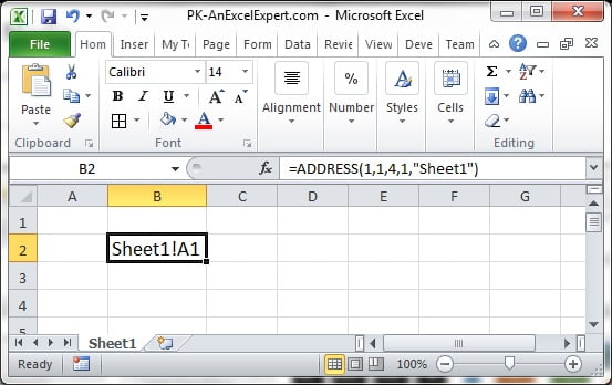
Row 2 uses the defaults, so the reference is absolute. Row 3 passes abs_num 4 for a relative reference. Row 4 switches to R1C1 notation. Row 5 shows that column 27 becomes AA. The screenshot below shows ADDRESS producing these text references for different row, column and abs_num settings.
Example 2: Find the cell that holds the highest sales figure
A sales list sits in A1:B6 with a header row. You want to tell the reviewer exactly which cell holds the maximum.
| A (Rep) | B (Sales) |
|---|---|
| Rep | Sales |
| Amit | 4,200 |
| Bela | 6,750 |
| Chen | 5,100 |
| Dana | 3,900 |
=ADDRESS(MATCH(MAX(B2:B5), B2:B5, 0) + 1, 2, 4)MATCH finds 6,750 in position 2 of B2:B5. Adding 1 corrects for the header row, so row_num is 3. Column 2 is B and abs_num 4 keeps it readable. The result is B3. Join it into a sentence with ="Top sales are in cell "&ADDRESS(...) for an audit note.
Example 3: Read any cell with ADDRESS and INDIRECT
Let a user type a row number in F1 and a column number in F2, then return the value at that position.
| Cell | Content | Formula | Result |
|---|---|---|---|
| F1 | 3 | =INDIRECT(ADDRESS(F1, F2)) |
6,750 (the value in B3) |
| F2 | 2 |
ADDRESS returns $B$3 as text and INDIRECT converts it into a live reference. The same result comes from =INDEX(A:B, F1, F2), which is faster on large workbooks because INDEX is not volatile.
Example 4: Convert a column number to a column letter
Excel has no built-in function for this, but ADDRESS and SUBSTITUTE do it in one line.
| A (Column number) | Formula in B | Result |
|---|---|---|
| 1 | =SUBSTITUTE(ADDRESS(1, A2, 4), "1", "") |
A |
| 27 | =SUBSTITUTE(ADDRESS(1, A3, 4), "1", "") |
AA |
| 702 | =SUBSTITUTE(ADDRESS(1, A4, 4), "1", "") |
ZZ |
ADDRESS builds a relative reference to row 1 of the column (for example AA1), and SUBSTITUTE removes the 1, leaving the letters.
Example 5: Reference a cell on another sheet
=ADDRESS(5, 4, 1, TRUE, "Summary")
=ADDRESS(1, 1, 4, TRUE, "Q1 Data")
The first formula returns Summary!$D$5. The second returns ‘Q1 Data’!A1, and ADDRESS adds the single quotes because the sheet name contains a space. Wrap either in INDIRECT to fetch the value. This is handy when a dashboard cell should pull from whichever sheet name a user picks from a drop-down list.
Tips and common mistakes
- Feed the numbers from formulas. Use ROW, COLUMN or MATCH for row_num and column_num so the address moves with the data when rows are inserted.
- Use abs_num 4 for anything users read. B3 is easier to read in a message than $B$3.
- Remember the result is text. ADDRESS(3, 2) + 1 gives #VALUE!. To use the cell value, wrap it in INDIRECT or switch to INDEX.
- Do not add your own quotes to sheet names. ADDRESS quotes names with spaces automatically; adding extra quotes produces a broken reference.
- Limit ADDRESS + INDIRECT pairs. INDIRECT is volatile and recalculates on every change. Hundreds of them slow a workbook noticeably.
- Check the abs_num range. Only 1 to 4 are valid; 0 or 5 returns #VALUE!.
- R1C1 output needs R1C1 consumers. INDIRECT reads R1C1 text only when its second argument is FALSE:
=INDIRECT(ADDRESS(3, 2, 1, FALSE), FALSE).
Errors and how to fix them
| Error | Cause | Fix |
|---|---|---|
| #VALUE! | row_num or column_num is 0, negative, text or larger than the sheet (1,048,576 rows, 16,384 columns); or abs_num is outside 1 to 4. | Check the inputs with ISNUMBER, and make sure a MATCH feeding the row has found a result. |
| #N/A | A MATCH inside ADDRESS did not find the lookup value. | Correct the lookup value or wrap the formula in IFERROR. |
| #REF! after INDIRECT | The text address points to a sheet that does not exist or is misspelt. | Check sheet_text against the tab name exactly, including spaces. |
| #NAME? | The function name is misspelt, or sheet_text was typed without quotes. | Type ADDRESS and put sheet names in double quotes. |
| Result shows $B$3 but you expected a value | ADDRESS returns text by design. | Use INDIRECT(ADDRESS(…)) or INDEX(range, row, col). |
Practice exercise
- Type 10 in A1 and 5 in B1. In C1 write a formula that returns E10 (relative style). Expected: E10.
- Change the same formula to return the R1C1 form. Expected: R10C5.
- Using the sales table from Example 2, write a formula that returns the address of the lowest sales figure. Expected: B5.
- Write a formula that converts the number 100 into its column letters. Expected: CV.
- Build a reference to cell C7 on a sheet called Monthly Report and wrap it in INDIRECT. Expected: the value in ‘Monthly Report’!C7.
Key takeaways
- ADDRESS turns a row number and a column number into a reference written as text.
- abs_num controls the dollar signs (1 to 4) and a1 switches between A1 and R1C1 styles.
- sheet_text adds a sheet prefix and quotes names with spaces for you.
- Combine ADDRESS with MATCH to report where a value sits, and with SUBSTITUTE to convert column numbers to letters.
- To read the value at the address, use INDIRECT sparingly or prefer the non-volatile INDEX.
Related functions and lessons
- Excel Formulas and Functions hub: every function lesson in module 5.
- INDIRECT: converts the text that ADDRESS builds into a live reference.
- ROW and COLUMN: supply the row and column numbers ADDRESS needs.
- INDEX: returns the value at a row and column position without building text, and is the faster choice when you only need the value.
- CELL: returns the address and other properties of an existing reference, the reverse of ADDRESS.
- OFFSET: another way to build references that move with your data.
- Excel Dashboard course: see how dynamic references drive interactive reports.
- Common errors in Excel formulas and how to fix them.
- Microsoft documentation: ADDRESS function.
Frequently asked questions
What does the abs_num argument do in ADDRESS?
abs_num sets the reference style of the text that ADDRESS returns. 1 (the default) gives an absolute reference such as $B$3, 2 gives A$1 style with only the row locked, 3 gives $A1 style with only the column locked, and 4 gives a plain relative reference such as B3. Any other number returns #VALUE!.
Can ADDRESS return an R1C1-style reference?
Yes. Set the fourth argument, a1, to FALSE. For example =ADDRESS(3, 2, 1, FALSE) returns R3C2, meaning row 3, column 2. If you later pass that text to INDIRECT, set the second argument of INDIRECT to FALSE as well so that it reads R1C1 notation.
How do I get the value of the cell that ADDRESS points to?
Wrap ADDRESS in INDIRECT: =INDIRECT(ADDRESS(3, 2)) returns the content of B3. INDIRECT is volatile, so on large sheets prefer =INDEX(A:Z, 3, 2), which returns the same value using the same row and column numbers without recalculating on every change.
How do I convert a column number to a column letter in Excel?
Use =SUBSTITUTE(ADDRESS(1, n, 4), “1”, “”), replacing n with the column number. ADDRESS builds a reference to row 1 of that column, for example AA1, and SUBSTITUTE removes the row number, leaving AA. It works for every column up to XFD.
Is ADDRESS a volatile function?
No. ADDRESS recalculates only when its arguments change. The performance concern comes from INDIRECT, which is volatile and recalculates whenever anything in the workbook changes. If you combine the two in many cells, consider replacing the pair with INDEX, which is not volatile.
Want the finished version? Ready-made Excel dashboards, trackers and VBA systems built with these functions are available at NextGenTemplates.com.