Part of the free Module 5: Excel Formulas and Functions · Function 40 of 105 · Full Excel course
The Excel INDEX function returns the value at a given row and column position inside a range or array. Tell INDEX where the data is and which row (and optionally column) you want, and it returns that cell’s content. Paired with MATCH, INDEX in Excel becomes a flexible lookup that works in any direction.
INDEX syntax
=INDEX(array, row_num, [column_num])
=INDEX(reference, row_num, [column_num], [area_num])
The first form (array form) covers almost every real-world use. The reference form lets you supply several ranges and pick one with area_num.
Arguments
| Argument | Required | Meaning |
|---|---|---|
| array | Required | The range or array constant to read from, for example A2:D50. |
| row_num | Required | The row position inside the range (1 = first row of the range, not row 1 of the sheet). Use 0 to return the whole column. |
| column_num | Optional | The column position inside the range. Omit it for a single-column range. Use 0 to return the whole row. |
| area_num | Optional | Reference form only: which of the supplied ranges to use, e.g. (A1:B5, D1:E5) with area_num 2 reads D1:E5. |
INDEX returns any data type: text, numbers, dates or logical values. It actually returns a reference, which is why it can also feed range-based functions such as SUM.
Step-by-step example
Assume a sales table in A2:D8 with Region, Product, Quantity and Amount. To fetch the Amount (column 4) from the third row of the table:
=INDEX(A2:D8, 3, 4)- Excel treats A2:D8 as a grid of 7 rows and 4 columns.
- It goes down to the 3rd row of that grid (sheet row 4).
- It moves across to the 4th column (column D) and returns D4.
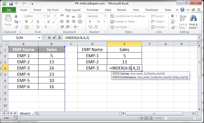
The screenshot below demonstrates INDEX picking a value from a table by row and column number.
Practical use cases
1. INDEX-MATCH: the flexible lookup
Let MATCH find the row, then let INDEX return the value from any column, including columns to the left of the lookup column:
=INDEX($D$2:$D$500, MATCH(G2, $A$2:$A$500, 0))Unlike VLOOKUP, this formula keeps working if you insert or delete columns, and it evaluates faster on large tables because it reads only one column.
2. Two-way lookup (row and column)
=INDEX($B$2:$M$20, MATCH($P2, $A$2:$A$20, 0), MATCH(Q$1, $B$1:$M$1, 0))Ideal for a month-by-product matrix: the first MATCH finds the product row, the second finds the month column.
3. Sum an entire column chosen by name
=SUM(INDEX($B$2:$M$20, 0, MATCH("Mar", $B$1:$M$1, 0)))Because row_num is 0, INDEX returns the whole column, which SUM then totals.
4. Last value in a list
=INDEX(A:A, COUNTA(A:A))XLOOKUP note: In Excel 365 and 2021, =XLOOKUP(G2, A2:A500, D2:D500) replaces the INDEX-MATCH pair in one step. INDEX-MATCH remains the compatible choice for workbooks opened in older versions.
Common mistakes and errors
- #REF! – row_num or column_num is outside the range (for example asking for row 10 of a 7-row range). Check the size of array.
- #VALUE! – row_num or column_num is text or a decimal that cannot be interpreted as a position.
- #N/A – comes from a nested MATCH that found nothing, not from INDEX itself. Wrap the formula in IFERROR or IFNA.
- Counting sheet rows instead of range rows – INDEX(A5:A20, 3) returns A7, not A3. Positions are always relative to the range.
- Relative references shift when copied – lock the array with $ signs before filling down.
Related functions
- MATCH – finds the position that INDEX needs.
- VLOOKUP – the simpler one-direction lookup.
- OFFSET – another way to build dynamic references.
- CHOOSE – picks one value from a list by position.
- See all lessons in the Excel Formulas hub.
Frequently asked questions
What is the difference between INDEX and VLOOKUP?
VLOOKUP searches for a value and can only return columns to its right. INDEX returns a value by position and, combined with MATCH, can look in any direction and is not broken by inserted columns.
Is INDEX-MATCH faster than VLOOKUP?
Yes, on large tables. INDEX-MATCH reads only the lookup column and the return column, while VLOOKUP loads the whole table_array for every formula.
Can INDEX return a whole row or column?
Yes. Set row_num to 0 to return the entire column, or column_num to 0 to return the entire row, then pass the result to SUM, AVERAGE or another function.
Need a ready-made template? Browse 7,000+ Excel, Power BI and Google Sheets templates at NextGenTemplates.com.