Part of the free Module 5: Excel Formulas and Functions · Function 41 of 105 · Full Excel course
Updated on 5 September 2026 · Works in Excel 365, 2021, 2019 and 2016 (and earlier).
The Excel INDIRECT function converts a text string into a live cell or range reference and returns whatever that reference contains. Use INDIRECT in Excel when the address you need is stored as text in another cell, when a formula must switch between worksheets by name, or when you want a reference that does not move when rows and columns are inserted.
INDIRECT syntax
=INDIRECT(ref_text, [a1])| Argument | Required or optional | What it does | Notes and defaults |
|---|---|---|---|
ref_text |
Required | A text string that describes a reference: a cell address such as “B5”, a range such as “Sheet2!A1:A10”, a defined name, or a cell that contains such text. | Text must describe a reference in an open workbook. A reference to a closed workbook returns #REF!. |
a1 |
Optional | Tells Excel which reference style the text uses. | TRUE or omitted: A1 style (for example B5). FALSE: R1C1 style (for example R5C2). |
How INDIRECT works
INDIRECT does not return a value of its own. It returns a reference, and Excel then evaluates that reference. Typed alone in a cell it shows the referenced value; placed inside SUM, VLOOKUP, COUNTIF or INDEX it supplies the range those functions read from. Because the address is built from text, Excel does not adjust it when you insert or delete rows, which is either a feature or a trap depending on what you intend.
INDIRECT is volatile: it recalculates every time anything in the workbook changes, not just when its inputs change. A handful of INDIRECT formulas are harmless; several thousand of them can make a workbook noticeably slow.
Version notes. INDIRECT behaves identically in Excel 365, 2021, 2019, 2016 and earlier. In Excel 365 a range returned by INDIRECT spills automatically if you type it as a plain formula, for example =INDIRECT("A1:A5"). Google Sheets has the same function with the same arguments. Non-volatile alternatives are INDEX, CHOOSE and, for consolidating sheets, Power Query.
Worked examples
Example 1: Turn a text address into a value
Cell A1 holds the text B5, and B5 holds 250. INDIRECT reads the text, treats it as an address and returns the value stored there.
| Cell | Content | Formula | Result |
|---|---|---|---|
| A1 | B5 | ||
| B5 | 250 | ||
| C1 | =INDIRECT(A1) |
250 | |
| C2 | =INDIRECT("B"&5) |
250 |
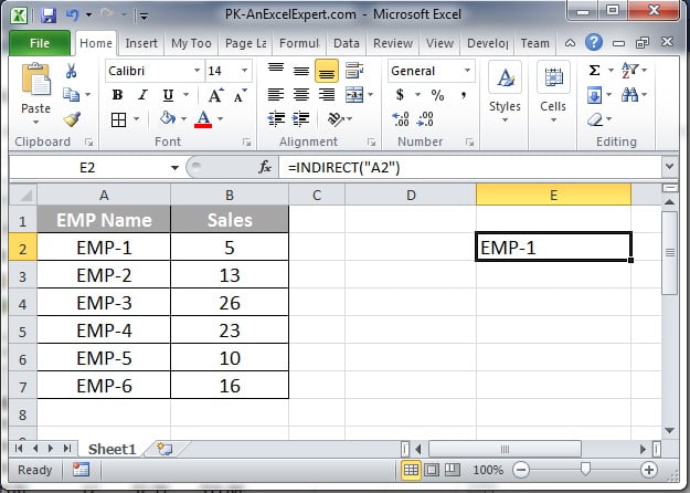
Change A1 to C7 and C1 immediately shows the content of C7. The screenshot below shows the same idea on a small sheet.
Example 2: Pull the same cell from many monthly sheets
A workbook has sheets named Jan, Feb, Mar and so on, each with the month total in D10. A summary sheet lists the sheet names in column A. One formula, copied down, collects every total.
| A (sheet name) | Formula in B | Result |
|---|---|---|
| Jan | =INDIRECT("'"&A2&"'!D10") |
Value of Jan!D10 |
| Feb | =INDIRECT("'"&A3&"'!D10") |
Value of Feb!D10 |
| Mar | =INDIRECT("'"&A4&"'!D10") |
Value of Mar!D10 |
The single quotes around the sheet name are essential: without them a sheet called “Q1 Sales” or one that starts with a digit produces #REF!.
Example 3: Dependent drop-down lists with Data Validation
Create a named range for each category, using the category text as the name (Fruits, Vegetables). Cell B2 holds a drop-down of the category names. The second drop-down in C2 uses this Data Validation list source:
=INDIRECT($B$2)| Named range | Contents | Selection in B2 | List shown in C2 |
|---|---|---|---|
| Fruits | Apple, Banana, Mango | Fruits | Apple, Banana, Mango |
| Vegetables | Carrot, Onion, Spinach | Vegetables | Carrot, Onion, Spinach |
Named ranges cannot contain spaces, so a category such as “Dry Fruits” needs SUBSTITUTE: =INDIRECT(SUBSTITUTE($B$2," ","_")) with the range named Dry_Fruits.
Example 4: Sum a column chosen by its letter
Cell F1 holds a column letter typed by the user. The formula totals rows 2 to 100 of that column.
| F1 | Formula | Reference built | Result |
|---|---|---|---|
| D | =SUM(INDIRECT(F1&"2:"&F1&"100")) |
D2:D100 | Total of D2:D100 |
| G | =SUM(INDIRECT(F1&"2:"&F1&"100")) |
G2:G100 | Total of G2:G100 |
Combine INDIRECT with COUNTA to make the range grow with the data: =SUM(INDIRECT(F1&"2:"&F1&COUNTA(A:A))).
Example 5: R1C1 style with numeric row and column
When the row and column are numbers rather than letters, R1C1 style avoids converting a column number to a letter. G1 holds the row number 5 and G2 the column number 2.
=INDIRECT("R"&G1&"C"&G2, FALSE)This returns the value in row 5, column 2, which is B5. The same result with INDEX is =INDEX(1:1048576, G1, G2), and INDEX is not volatile, so prefer it in large models.
Tips and common mistakes
- Quote sheet names. Always build references as
"'"&name&"'!A1"; the quotes are harmless for simple names and required for names with spaces or leading digits. - Use a drop-down for the sheet name input. A Data Validation list of sheet names stops users from mistyping and producing #REF!.
- Test the reference first.
=IF(ISREF(INDIRECT(A1)), INDIRECT(A1), "Sheet missing")returns a friendly message instead of an error. - Keep INDIRECT out of large tables. It is volatile. Use INDEX, CHOOSE or structured Table references where the set of ranges is fixed.
- Closed workbooks do not work. INDIRECT reads only open workbooks. For closed files use a direct external link or Power Query.
- Remember the address never shifts. Inserting a row above B5 does not turn
=INDIRECT("B5")into B6. Use this deliberately for anchored references, and avoid it when the data moves. - Do not pass a bare address.
=INDIRECT(B5)reads the text inside B5;=INDIRECT("B5")reads B5 itself. Mixing these up is the most common beginner error.
Errors and how to fix them
| Error | Cause | Fix |
|---|---|---|
| #REF! | ref_text is not a valid reference: misspelt sheet name, missing single quotes, deleted named range, reference beyond the sheet limits, or a closed external workbook. | Check the text with a helper cell, add the quotes, recreate the name, or open the source workbook. |
| #NAME? | The text was typed without quotation marks, so Excel treats it as an undefined name, or the function is misspelt. | Wrap literal addresses in quotes: =INDIRECT("B5"). |
| #VALUE! | ref_text refers to a whole multi-cell range but the formula sits in a single cell in Excel 2019 or earlier, or a1 is a non-logical value. | Wrap in an aggregating function such as SUM, or use TRUE/FALSE for a1. |
| #SPILL! | In Excel 365 the returned range needs more cells than are free below or to the right. | Clear the blocking cells or wrap INDIRECT in a function that returns one value. |
| Wrong value, no error | The text builds a valid address but not the one you intended, often after rows were inserted. | Show the built text in a helper cell to verify it before passing it to INDIRECT. |
Practice exercise
- Type any cell address in A1 and a number in that cell. Write
=INDIRECT(A1)in B1 and confirm it returns the number. Expected: changing A1 to another address changes B1 immediately. - Create three sheets named North, South and East with a total in cell C5 of each. On a summary sheet list the names in A2:A4 and use INDIRECT to fetch every C5. Expected: three totals without editing the formula per row.
- Build the dependent drop-down from Example 3 using two named ranges and Data Validation. Expected: the second list changes when the first selection changes.
- In F1 type a column letter and total that column with
=SUM(INDIRECT(F1&"2:"&F1&"50")). Expected: typing a different letter re-totals a different column. - Rewrite exercise 4 with INDEX and MATCH so the formula is not volatile. Expected: the same total with faster recalculation.
Key takeaways
- INDIRECT turns text into a reference; it is the bridge between a typed address and a working formula.
- Pass text inside quotes for a literal address, or a cell reference to read the address from that cell.
- Wrap sheet names in single quotes and never reference closed workbooks.
- INDIRECT is volatile, so use it sparingly in large workbooks and prefer INDEX or CHOOSE for fixed sets of ranges.
- Its best uses are dependent drop-downs, multi-sheet summaries and references that must not shift.
Related functions and lessons
- Excel Formulas and Functions library: every function page in this module.
- ADDRESS: builds the text address that INDIRECT can then read.
- OFFSET: another volatile function for dynamic ranges, better when the range moves by a number of rows or columns.
- INDEX: the non-volatile way to pick a cell or range by position.
- CHOOSE: picks one range from a short fixed list by number.
- ISREF: tests whether INDIRECT produced a valid reference.
- Data Validation course: build the drop-down lists used in Example 3.
- Microsoft Support: INDIRECT function.
Frequently asked questions
What is the INDIRECT function used for in Excel?
INDIRECT turns text such as Sheet2!B5 into a working reference. The most common uses are dependent drop-down lists, summary sheets that pull the same cell from many worksheets by name, formulas that total a column chosen by the user, and references that must stay fixed on a cell even when rows or columns are inserted above it.
Why does INDIRECT return #REF!?
The text does not describe a valid reference. Typical causes are a misspelt sheet name, a sheet name with spaces that is missing its single quotes, a named range that was deleted or renamed, or a reference to a workbook that is currently closed. Display the built text in a helper cell to see exactly what INDIRECT is trying to read.
Does INDIRECT work with closed workbooks?
No. INDIRECT can only read from workbooks that are open in the same Excel session. If the source file is closed the formula returns #REF!. For closed files use a normal external reference, which Excel caches, or import the data with Power Query, which is also much faster for consolidating many files.
Is INDIRECT slow?
INDIRECT is a volatile function, so it recalculates whenever anything in the workbook changes. A few dozen formulas make no difference, but thousands of them can make every edit sluggish. Where the set of possible ranges is fixed, INDEX or CHOOSE give the same result without volatility, and Tables with structured references remove the need altogether.
How do I use INDIRECT with a sheet name in a cell?
Concatenate the sheet name with the cell address and wrap the name in single quotes: =INDIRECT("'"&A2&"'!D10"). If A2 contains Jan, the formula reads Jan!D10. The quotes are required for names that contain spaces or start with a number, and they do no harm for simple names, so always include them.
Want the finished version? Ready-made Excel dashboards, trackers and VBA systems built with these functions are available at NextGenTemplates.com.