Part of the free Module 5: Excel Formulas and Functions · Function 9 of 105 · Full Excel course
Updated on 5 September 2026 · Works in Excel 365, 2021, 2019 and 2016 (and earlier).
The Excel CHOOSE function returns one value from a list of up to 254 values based on an index number. CHOOSE(2, “Red”, “Green”, “Blue”) returns Green. The values can be text, numbers, cell references, ranges or formulas, so CHOOSE in Excel is a compact way to map a number to a label, switch between scenarios in a model, or pick which range another function should work on, all without a lookup table.
CHOOSE syntax
=CHOOSE(index_num, value1, [value2], ...)| Argument | Required or optional | What it does | Notes and defaults |
|---|---|---|---|
| index_num | Required | Which value to return: 1 returns value1, 2 returns value2, and so on. | A number from 1 to 254, a cell reference or a formula that produces one. Decimals are truncated, so 2.9 becomes 2. Numbers below 1 or above the count of values return #VALUE!. An array such as {1,2} makes CHOOSE return several values at once. |
| value1 | Required | The item returned when index_num is 1. | Any constant, cell reference, range, named range or formula. Text must be in double quotes. |
| value2, … value254 | Optional | Further items returned for index_num 2, 3 and so on. | Up to 254 values in total. Each value may be a different type; CHOOSE does not require them to match. |
How CHOOSE works
CHOOSE evaluates index_num, counts along the list of values to that position and returns whatever it finds there. Only the selected value is calculated, so the other branches can be expensive formulas without slowing the sheet. When a value is a range reference, CHOOSE returns the reference itself, not a single cell. That is why CHOOSE can sit inside SUM, VLOOKUP or AVERAGE to switch the range those functions read.
Because index_num can be an array, CHOOSE({1,2}, C2:C10, A2:A10) builds a virtual two-column table on the fly. In Excel 365 that array spills; in older versions it is used inside another function such as VLOOKUP. CHOOSE is not volatile, which makes it a lighter alternative to INDIRECT for switching between ranges.
Version notes: CHOOSE works in every Excel version and in Google Sheets with the same syntax. Excel 2019 and later added SWITCH, which matches a value rather than a position and accepts a default. Excel 365 also has CHOOSECOLS and CHOOSEROWS for picking columns or rows out of an array, which is a different job from CHOOSE.
Worked examples
Example 1: Turn a weekday number into a day name
WEEKDAY returns 1 for Sunday through 7 for Saturday. CHOOSE converts that number into a label.
| A (Date) | Formula in B | Result |
|---|---|---|
| 01-Sep-2026 | =CHOOSE(WEEKDAY(A2), "Sun", "Mon", "Tue", "Wed", "Thu", "Fri", "Sat") |
Tue |
| 05-Sep-2026 | same formula filled down | Sat |
| 06-Sep-2026 | same formula filled down | Sun |
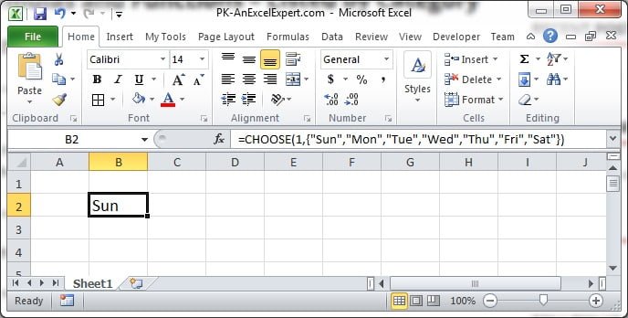
For 1 September 2026, WEEKDAY returns 3, so CHOOSE counts to the third value and returns Tue. The screenshot below shows CHOOSE returning items from a list according to the index number supplied.
Example 2: Convert a month into a fiscal quarter
A company year starts in April, so April to June is Q1. CHOOSE maps the twelve month numbers directly.
| A (Date) | MONTH(A) | Formula in B | Result |
|---|---|---|---|
| 15-Apr-2026 | 4 | ="Q"&CHOOSE(MONTH(A2), 4,4,4, 1,1,1, 2,2,2, 3,3,3) |
Q1 |
| 20-Nov-2026 | 11 | same formula | Q3 |
| 10-Feb-2027 | 2 | same formula | Q4 |
The list is written in month order (January first), so positions 1 to 3 return 4 for Q4, positions 4 to 6 return 1, and so on. For a calendar year, use =ROUNDUP(MONTH(A2)/3, 0) instead.
Example 3: Scenario switch in a financial model
Three forecast columns hold Base, Best and Worst revenue. A single cell, B1, chooses which one feeds the rest of the model.
| Scenario (B1) | C5 Base | D5 Best | E5 Worst | Formula in F5 | Result |
|---|---|---|---|---|---|
| 1 | 120,000 | 150,000 | 95,000 | =CHOOSE($B$1, C5, D5, E5) |
120,000 |
| 2 | 120,000 | 150,000 | 95,000 | same formula | 150,000 |
| 3 | 120,000 | 150,000 | 95,000 | same formula | 95,000 |
Add a data-validation drop-down on B1 with the values 1, 2 and 3, and label it Base, Best, Worst in the next cell, so users know what each number means. If you prefer the drop-down to show words, convert them with MATCH: =CHOOSE(MATCH($B$1, {"Base","Best","Worst"}, 0), C5, D5, E5).
Example 4: Pick a range for SUM
Three sheets hold monthly sales in B2:B50. Cell F1 holds a month number and one SUM formula totals the chosen sheet.
=SUM(CHOOSE(F1, Jan!B2:B50, Feb!B2:B50, Mar!B2:B50))CHOOSE returns the whole range from the selected sheet and SUM adds it. Unlike INDIRECT, this is not volatile and does not break if a sheet is renamed, because the references update automatically.
Example 5: VLOOKUP to the left with CHOOSE
VLOOKUP can only return columns to the right of the lookup column. CHOOSE with an array index builds a reversed table so it can look left.
| A (Employee ID) | B (Name) | C (Email) |
|---|---|---|
| E101 | Priya | priya@example.com |
| E102 | Rahul | rahul@example.com |
| E103 | Sara | sara@example.com |
=VLOOKUP("rahul@example.com", CHOOSE({1,2}, C2:C4, A2:A4), 2, FALSE)CHOOSE({1,2}, C2:C4, A2:A4) creates a two-column array with Email first and ID second, so VLOOKUP finds the email and returns E102. INDEX and MATCH, or XLOOKUP in Excel 365 and 2021, do the same job more readably; this pattern is useful when you must stay inside VLOOKUP.
Tips and common mistakes
- Keep lists short and stable. Weekdays, quarters and fixed scenarios suit CHOOSE. Anything that changes often belongs in a lookup table with VLOOKUP or XLOOKUP.
- Document what each index means. Put a legend next to the input cell or use a data-validation list so users never type 4 into a three-option switch.
- Use MATCH to accept words. CHOOSE(MATCH(F1, {“Low”,”Medium”,”High”}, 0), …) lets the user pick text while CHOOSE still receives a number.
- Prefer CHOOSE to INDIRECT for range switching. It is not volatile and survives sheet renames.
- Watch the argument order. Values are positional. If you insert a new option in the middle, every index number after it shifts.
- Guard calculated indexes. A formula that can return 0 or a number above the list length produces #VALUE!. Wrap it in MIN and MAX or check it with IF.
- Mixed types are fine. One value can be text, another a number and another a range; CHOOSE returns whatever sits at the chosen position.
Errors and how to fix them
| Error | Cause | Fix |
|---|---|---|
| #VALUE! | index_num is less than 1, greater than the number of values, or text such as “2” that Excel cannot convert. | Check the range of the index with =MAX(1, MIN(n, index)) or convert text with VALUE. |
| #NAME? | A text value is missing its double quotes, or the function name is misspelt. | Put every text constant in quotes. |
| #N/A | A MATCH used to build index_num found no match. | Correct the lookup value or add IFERROR around the MATCH. |
| #REF! | A range used as a value was deleted. | Repoint the reference. |
| Wrong item returned | Decimal index truncated (2.9 became 2) or the list order does not match the numbering. | Round the index with ROUND if needed and check the order of the values. |
Practice exercise
- In A1 type 3. In B1 write a CHOOSE formula that returns Gold for 1, Silver for 2 and Bronze for 3. Expected: Bronze.
- Put a date in A2 and write a formula that returns the full weekday name using WEEKDAY and CHOOSE. Expected: for 5 September 2026, Saturday.
- Write a formula that converts the month of a date into a calendar quarter label Q1 to Q4 using CHOOSE. Expected: for 20 November 2026, Q4.
- Create three columns of numbers and a scenario cell. Use CHOOSE to sum whichever column the scenario cell selects. Expected: the total of the chosen column.
- Using the employee table in Example 5, look up a name in column B and return the ID from column A with VLOOKUP and CHOOSE. Expected: for Sara, E103.
Key takeaways
- CHOOSE returns the value at the position given by index_num from a list of up to 254 values.
- Values can be constants, references, ranges or formulas, and only the chosen one is calculated.
- It is ideal for small fixed mappings (weekdays, quarters, scenarios) and for switching the range a SUM or VLOOKUP reads.
- An array index such as {1,2} builds a virtual table, which lets VLOOKUP look to the left.
- For longer or changing lists use a lookup table; for matching values rather than positions use SWITCH.
Related functions and lessons
- Excel Formulas and Functions hub: every function lesson in module 5.
- SWITCH: compares a value against a list of value and result pairs and accepts a default; use it when you match text rather than positions.
- INDEX: picks a value from a range by row and column, the better choice when the options live on the sheet.
- VLOOKUP and MATCH: table-based alternatives for longer lists.
- IFS: condition-based branching when the choice depends on tests rather than a number.
- Data Validation course: build the drop-down lists that drive a CHOOSE scenario switch.
- CHOOSE formula in Excel with examples (blog post).
- Microsoft documentation: CHOOSE function.
Frequently asked questions
Can CHOOSE return text and numbers in the same list?
Yes. The values can be any mix of text, numbers, dates, cell references, ranges or formulas. Text constants must be wrapped in double quotes, but there is no requirement for the values to share a type. CHOOSE simply returns whatever sits at the chosen position.
Can CHOOSE select values from other worksheets?
Yes. Use full references such as Sheet2!B5 or ‘Sales Data’!B2:B50 as the values, and each option can point to a different sheet. Combined with SUM or AVERAGE this lets one formula total whichever sheet a user selects, without the volatility of INDIRECT.
What is the difference between CHOOSE and SWITCH?
CHOOSE selects by position number only, so the input must be 1, 2, 3 and so on. SWITCH compares an expression with a list of specific values, returns the matching result and accepts a default when nothing matches. SWITCH is available in Excel 2019 and later; CHOOSE works in every version.
Why does my CHOOSE formula return #VALUE!?
Almost always because index_num is outside the list: 0, a negative number, or larger than the number of values you supplied. It also happens when index_num is text. Check the value feeding the index and limit it with MIN and MAX, or convert text to a number with VALUE.
How many values can CHOOSE hold?
Up to 254 values in Excel 2007 and later. In practice, lists longer than a dozen items are hard to read and maintain inside a formula, so move the options to a small table and use VLOOKUP, INDEX or XLOOKUP instead.
Want the finished version? Ready-made Excel dashboards, trackers and VBA systems built with these functions are available at NextGenTemplates.com.